• Portfolio
  • Aviation
  • Blog
  • About
Menu

David S Miller

  • Portfolio
  • Aviation
  • Blog
  • About
 The ConEd building is a historical landmark so the exterior masonry, etc. cannot be modified.

The ConEd building is a historical landmark so the exterior masonry, etc. cannot be modified.

 The interior is very modern, however.

The interior is very modern, however.

 BreakerBot sits on a sofa in the lobby.

BreakerBot sits on a sofa in the lobby.

 Setting up in the conference room

Setting up in the conference room

 Group photo after the presentation.

Group photo after the presentation.

 The ConEd building is a historical landmark so the exterior masonry, etc. cannot be modified.  The interior is very modern, however.  BreakerBot sits on a sofa in the lobby.  Setting up in the conference room  Group photo after the presentation.

BreakerBot Moves to ConEdison

May 25, 2016

Yesterday we visited ConEdison in my hometown of NYC to present our Senior Capstone project, BreakerBot. The goal of this phase of the project was to convince ConEd to continue future phases of the project at BU by delivering a prototype that could:

  1. Automatically align to the front of the cubicle where the breaker is located

  2. Automatically remove the breaker from the cubicle and reinsert it once aligned

We demonstrated these functions for them with our prototype, and we had a long conversation about the technical and logistical constraints that would need to be considered and accounted for in a full scale robot. As for sealing ConEd's commitment for next year, we are still working on the business aspect of the deal and that's really all I can say right now. 

We did leave BreakerBot there so that it could be used to help secure funding for the project from the higher-ups who were unable to attend our presentation. It was hard to say goodbye to BreakerBot, but we are very happy to know that BreakerBot has a new home at ConEd. 

$\setCounter{0}$
In Academic Projects, BreakerBot Tags BreakerBot
Comment
 Always use vector image formats (PNG, TIF, etc.) to ensure crisp resolution at any scale.

Always use vector image formats (PNG, TIF, etc.) to ensure crisp resolution at any scale.

 Aluminum standoff spacers

Aluminum standoff spacers

 They have an additional function to prevent the swerve modules from crashing into the plaque when the robot steers...

They have an additional function to prevent the swerve modules from crashing into the plaque when the robot steers...

 BreakerBot looking good! We have to do something about its hair though

BreakerBot looking good! We have to do something about its hair though

 Always use vector image formats (PNG, TIF, etc.) to ensure crisp resolution at any scale.  Aluminum standoff spacers  They have an additional function to prevent the swerve modules from crashing into the plaque when the robot steers...  BreakerBot looking good! We have to do something about its hair though

BreakerBot Gets a New Look

May 11, 2016

Even though our senior design class is technically over, we still have some things to finish with our project. We are traveling to my hometown of New York City to give a presentation and demonstration of our robot at ConEd. The goal of this is to convince them to continue future phases of the project at BU to design and build a full scale version of the robot. 

We spent the day trying to make our robot look a bit more professional and presentable by adding lasercut acrylic plaques of our sponsors' logos. We also turned some aluminum standoff spacers that I think add a really nice touch.

$\setCounter{0}$
In Academic Projects, BreakerBot, Machining Projects Tags BreakerBot, Lasercutting, Machining
Comment
IMG_7481_2.JPG
IMG_7483.jpg
IMG_7481_2.JPG IMG_7483.jpg

BreakerBot Wins an Award

May 4, 2016

Yesterday our team had our senior design presentation for our BreakerBot project. We ended up winning the Best Senior Project award from the BU Department of Electrical and Computer Engineering. I also won two personal awards that day for my design portfolio on this website!

$\setCounter{0}$
In Academic Projects, BreakerBot Tags Award
Comment
 +Y translation + CW rotation. Notice the skidding. If the X vel. were +, the motion would be correct. I hadn't fixed the wheel angles at this point though; those are still wrong.

+Y translation + CW rotation. Notice the skidding. If the X vel. were +, the motion would be correct. I hadn't fixed the wheel angles at this point though; those are still wrong.

 Pure translation in Q1. Notice the X velocity still seems to have the wrong sign.

Pure translation in Q1. Notice the X velocity still seems to have the wrong sign.

 I don't remember what this is. I don't think it worked...

I don't remember what this is. I don't think it worked...

 This looks correct, but it's not. If you try gradually reducing the rotation and keeping the translation the same, you'll notice something wrong. It's helpful to test limiting cases like this, by introducing things very slowly. 

This looks correct, but it's not. If you try gradually reducing the rotation and keeping the translation the same, you'll notice something wrong. It's helpful to test limiting cases like this, by introducing things very slowly. 

 I stopped doing the motion plots and just did a single snapshot with velocity vectors. You have to adjust the sign of the wheel velocity to get the vector pointing in the right direction.

I stopped doing the motion plots and just did a single snapshot with velocity vectors. You have to adjust the sign of the wheel velocity to get the vector pointing in the right direction.

 Here you can see all the wheels have the same velocity [vector] as each other, and as the body of the robot. Bingo.

Here you can see all the wheels have the same velocity [vector] as each other, and as the body of the robot. Bingo.

 Here's where I started trying to combine translation inputs and rotation inputs. Here the robot has a Y+ translation and a CCW rotation. The net result is a pure rotation about some point on the X axis.

Here's where I started trying to combine translation inputs and rotation inputs. Here the robot has a Y+ translation and a CCW rotation. The net result is a pure rotation about some point on the X axis.

 Now I'm combining X and Y translation with rotations. I repeated this for different quadrants (translation) and different rotation directions (CW,CCW). 

Now I'm combining X and Y translation with rotations. I repeated this for different quadrants (translation) and different rotation directions (CW,CCW). 

 You can see that the lower left wheel is on the largest radius of the orbit, and it has the highest speed. Good sign.

You can see that the lower left wheel is on the largest radius of the orbit, and it has the highest speed. Good sign.

 I went through each translational quadrant twice, one for each rotation direction (CW,CCW). 

I went through each translational quadrant twice, one for each rotation direction (CW,CCW). 

 One other verification I could do is making sure the normal lines from each wheel intersect at the same point. This is the orbital point I mentioned in the text below. 

One other verification I could do is making sure the normal lines from each wheel intersect at the same point. This is the orbital point I mentioned in the text below. 

success_5.png
success_4.png
success_3.png
success_2.png
 +Y translation + CW rotation. Notice the skidding. If the X vel. were +, the motion would be correct. I hadn't fixed the wheel angles at this point though; those are still wrong.  Pure translation in Q1. Notice the X velocity still seems to have the wrong sign.  I don't remember what this is. I don't think it worked...  This looks correct, but it's not. If you try gradually reducing the rotation and keeping the translation the same, you'll notice something wrong. It's helpful to test limiting cases like this, by introducing things very slowly.   I stopped doing the motion plots and just did a single snapshot with velocity vectors. You have to adjust the sign of the wheel velocity to get the vector pointing in the right direction.  Here you can see all the wheels have the same velocity [vector] as each other, and as the body of the robot. Bingo.  Here's where I started trying to combine translation inputs and rotation inputs. Here the robot has a Y+ translation and a CCW rotation. The net result is a pure rotation about some point on the X axis.  Now I'm combining X and Y translation with rotations. I repeated this for different quadrants (translation) and different rotation directions (CW,CCW).   You can see that the lower left wheel is on the largest radius of the orbit, and it has the highest speed. Good sign.  I went through each translational quadrant twice, one for each rotation direction (CW,CCW).   One other verification I could do is making sure the normal lines from each wheel intersect at the same point. This is the orbital point I mentioned in the text below.  success_5.png success_4.png success_3.png success_2.png

Kinematics of Wheeled Mobile Robots Pt. 3

April 14, 2016

Our team finally got the robot moving and steering! Which means it's finally time for me to start the implementation process of the kinematic and control equations. To further verify and help prepare for the implementation, I made a little simulator in MATLAB to help visualize how the robot will move given certain (steady state) commands. Transient commands are a whole other issue, which I may discuss later. 

The structure of the top level code is simple. It defines the parameters of the robot and of the simulation, and calls the swerve_command function. This function performs the inverse kinematics and spits out the wheel angles and speeds, as well as the position (x, y, theta) information for that time step. Over several time steps, the robot will move. If steady state inputs are held, the wheel angles and speeds will remain constant, even if the robot itself is executing some curvilinear motion. The robot is plotted at each time step. To verify the wheel angles are correct, you need to visually confirm that the wheels are tangent to the path taken by the wheels in each snapshot. 

Confirming the wheel speeds is more difficult. For any type of pure translation all the wheel speeds just need to be the same. This has been confirmed. If there is any type of rotation involved, the wheels will orbiting some central point. If the location of the point is known, then the radius to each wheel can be found and using the omega = v/r equation you can confirm that all the angular speeds about that central point are equal. This is hard to do currently because we are normalizing all our speeds because they are simply throttling values which will be sent to the motors. We do not know exactly what speeds they will spin at. However, the ratios of the speeds are telling. What we know is that the wheels on the largest radius of the orbit must have the highest linear velocity, and the wheels on the smallest radius of the orbit must have the smallest linear velocity. This allows all the wheels to have the same angular velocity around that central point. As you can see from the photos, this phenomenon is evident by the colored velocity vectors. 

There is something funky going on with the way that the motion of the robot is plotted. The wheel angles and speeds look okay, but when I try to plot the motion some of the components of the motion (X and rotation) have the wrong sign and it looks like the robot is skidding across the floor. I haven't been able to figure out why that is yet. I have a feeling it's some kind of sign error but I haven't found it yet.


Open Issues:

  1. Figuring out how to update the wheel speeds and angles while moving (transient command inputs)

  2. Normalizing the wheel speed outputs to prevent speed commands to the motor from saturating

  3. Finding the little sign errors that are messing things up


Bonus:

We also made a little case for the webcam BreakerBot will be using for the First Person View mode for remote operation. BreakerBot is watching you...

$\setCounter{0}$
In Academic Projects, BreakerBot, MATLAB Projects Tags MATLAB, kinematics, Modeling
Comment
 It appears that this mechanism is valid... But how can I be sure?

It appears that this mechanism is valid... But how can I be sure?

 By plotting arcs around the links I ensure they stay the same size throughout.

By plotting arcs around the links I ensure they stay the same size throughout.

 Here are some varying geometries that achieve the same goal.

Here are some varying geometries that achieve the same goal.

 This is when I was still debugging my code. You can clearly see each member changes length as it rotates, which cannot occur.

This is when I was still debugging my code. You can clearly see each member changes length as it rotates, which cannot occur.

 This geometry resulted in a bearing that was placed off the surface of the shipping container.

This geometry resulted in a bearing that was placed off the surface of the shipping container.

 One more geometry. The next question is, how can you optimize the linkage??

One more geometry. The next question is, how can you optimize the linkage??

 I tried plotting snapshots of the linkage but it didn't work so well. This is wrong because the magenta snapshots do not align with the red position.

I tried plotting snapshots of the linkage but it didn't work so well. This is wrong because the magenta snapshots do not align with the red position.

 It appears that this mechanism is valid... But how can I be sure?  By plotting arcs around the links I ensure they stay the same size throughout.  Here are some varying geometries that achieve the same goal.  This is when I was still debugging my code. You can clearly see each member changes length as it rotates, which cannot occur.  This geometry resulted in a bearing that was placed off the surface of the shipping container.  One more geometry. The next question is, how can you optimize the linkage??  I tried plotting snapshots of the linkage but it didn't work so well. This is wrong because the magenta snapshots do not align with the red position.

MATLAB Four-Bar Linkage Design

March 24, 2016

The Product Design class I am a TA for had an assignment to design a four-bar mechanism to move a lid on a shipping container up and over so that it rested on the top of the container during loading. There was extra credit awarded to those who could analytically arrive at a design using MATLAB (or some other language). I made my own solution for fun and to check student's solutions. I tried to get it to plot each snapshot (in magenta) but it was not correct and I didn't have time to figure it out. 

So, here's how to design a typical four-bar linkage:

  1. Define the desired locations of your coupler. You define two or three locations you want the coupler to travel through. My code only works with three locations.

  2. Find the locus of points that is equidistant from where the crank connects to the coupler in each position. If two coupler positions are defined, the locus will be an infinite line (think of the intersection of two circles; connecting the two points forms a line). If three coupler positions are defined, the locus collapses to a single point. This point also happens to be the circumcenter of the triangle formed by the three vertices the bearing must be equidistant from. The bearing must be placed on a point on the locus. If the locus is a single point, your job is done. If the locus is a line, you must select a point on that line to be your bearing location.

  3. Repeat step 2 for the points where the rocker connects to the coupler.

  4. Once you have the bearing locations for the crank and the rocker, you can easily calculate the lengths of each link.

$\setCounter{0}$
In Academic Projects, Personal Projects, MATLAB Projects Tags MATLAB, kinematics, Mechanisms
Comment
 User interface for the GUI.

User interface for the GUI.

 This plot shows where all the loft curves are located relative to each other. This allows the user to confirm that all the components are in the right place relative to each other before exporting all the curves as text files.

This plot shows where all the loft curves are located relative to each other. This allows the user to confirm that all the components are in the right place relative to each other before exporting all the curves as text files.

 User interface for the GUI.  This plot shows where all the loft curves are located relative to each other. This allows the user to confirm that all the components are in the right place relative to each other before exporting all the curves as text files.

MATLAB Project: Aircraft Designer

November 5, 2015

This is the master program which all the functions described in previous posts feed into. This takes inputs from the fuselage designer, wing designer, and empennage designer and puts all the components together. The motivation for this project was to be able to quickly and easily iterate through aircraft designs. All of the performance calculations were done in an excel spreadsheet, but Excel is not good at making custom plots or managing data. This program receives the geometric parameters of the airplane calculated by the Excel sheet, and uses them to 'build' the airplane for visualization and accurate component layout.

The component layout in the spreadsheet does not account for the form of the volume components (passenger cabin, cockpit, galley, wing box, etc.). On more than one occasion we had designed a fuselage that seemed to contain all the components, only to realize that the calculated cabin length was longer than the fuselage of the aircraft! This program was intended to solve that problem by visualizing the components for instantaneous feedback on the quality of the layout. 

The other main goal of the program was to facilitate the rapid 3-D modeling of the aircraft. Unlike most other objects undergraduates are used to CADing, aircraft often have complex curvatures and geometries that take a long time to make manually. This program produces curves for the fuselage, main wing, and tail surfaces and positions them according to the design specifications. The coordinates for the curves are then exported as .txt files, which can be uploaded into SolidWorks as curves and lofted together. This drastically reduces the time required to produce a solid model and thus enables more rapid design iteration and evaluation.

I'd like to continue adding more to this program, but it looks like there simply isn't enough room on the UI to add more input boxes. Already, many of the parameters cannot be changed from the UI; the code must be manually altered. I was thinking of adding tabbed panels to increase the number of inputs possible, but from my [limited] research they don't seem to be well supported. I think this version should do for now.

$\setCounter{0}$
In Academic Projects, MATLAB Projects Tags MATLAB, Aerospace, Aircraft Design
Comment
 A four bladed propeller with 10ft diameter and an activity factor of 140, similar to what might be seen on the LAS Anthony.

A four bladed propeller with 10ft diameter and an activity factor of 140, similar to what might be seen on the LAS Anthony.

 A jet engine fan blade isn't that much different than a propeller blade when you get down to it... But this is just for show!

A jet engine fan blade isn't that much different than a propeller blade when you get down to it... But this is just for show!

 A four bladed propeller with 10ft diameter and an activity factor of 140, similar to what might be seen on the LAS Anthony.  A jet engine fan blade isn't that much different than a propeller blade when you get down to it... But this is just for show!

MATLAB Mini Project: Propeller Design

November 5, 2015

As part of my ongoing aircraft design project, I wrote another MATLAB function to produce propellers whose cross sections could be exported for making models in SolidWorks. The function takes inputs from the design calculations of an Excel spreadsheet. The diameter of the rotor, the number of blades, the twist of the blade, and the airfoils comprising the blade are all used to determine the shape of the propeller. For now, only straight tapered blades defined by a root and tip airfoil can be produced. But this code serves as a first step for designing and plotting more complicated blades with curved planforms and nonlinear twists. Right now the twists are user defined, whereas in reality the twist is set to produce a certain coefficient of lift stated in the Hamilton Standard propeller efficiency chart; this is something else that must be accounted for in the future.

I considered having this function calculate all performance parameters of the propeller, but the only performance estimation method that seemed feasible was the blade element method. This method is far less accurate than the Hamilton Standard propeller efficiency charts used to calculate performance in the Excel sheet. So I decided to stick with the standard method of propeller sizing using the propeller charts and just let my program calculate the propeller's shape.

$\setCounter{0}$
In Academic Projects, MATLAB Projects Tags MATLAB, Propeller, Aircraft Design
1 Comment
Screen Shot 2015-10-12 at 12.52.21 PM.png
 I added another axis to plot the side view and centerline. This is to make sure the nose and tail are offset from the centerline correctly.

I added another axis to plot the side view and centerline. This is to make sure the nose and tail are offset from the centerline correctly.

 Can now also plot internal layout of pax seats, cockpit, lavatory, and galley. These locations will come in useful for calculating center of mass and longitudinal stability later.

Can now also plot internal layout of pax seats, cockpit, lavatory, and galley. These locations will come in useful for calculating center of mass and longitudinal stability later.

 Area vs Length plot for Area Ruling. I havent accounted for wing/engine area yet; this is just the fuselage.

Area vs Length plot for Area Ruling. I havent accounted for wing/engine area yet; this is just the fuselage.

1st image.png
Screen Shot 2015-10-12 at 12.52.21 PM.png  I added another axis to plot the side view and centerline. This is to make sure the nose and tail are offset from the centerline correctly.  Can now also plot internal layout of pax seats, cockpit, lavatory, and galley. These locations will come in useful for calculating center of mass and longitudinal stability later.  Area vs Length plot for Area Ruling. I havent accounted for wing/engine area yet; this is just the fuselage. 1st image.png

MATLAB Project: Fuselage Designer

October 12, 2015

This project builds off my previous MATLAB project for designing and making wings in CAD. I have added basic fuselage plotting capabilities. The user simply defines the maximum diameter and fineness ratios to determine the fuselage length. Then, 11 cross sections are defined by their widths and heights. The shapes of the cross sections are assumed to be ellipses. The tail angle can also be changed. Wing twist has also been added; root and chord angles can now be set.


10/14/15 - Added 3 additional plots: fuselage side view, top view, and max diameter section view. The program can now display seating arrangements, galley, and lavatory locations.

$\setCounter{0}$
In Academic Projects, MATLAB Projects Tags MATLAB, Aircraft Design, Fuselage
Comment
 Jet transport wing.

Jet transport wing.

 Regional turboprop wing

Regional turboprop wing

 Supersonic delta wing

Supersonic delta wing

 4 seat GA wing (C172)

4 seat GA wing (C172)

 Jet transport wing.  Regional turboprop wing  Supersonic delta wing  4 seat GA wing (C172)

MATLAB Project: Wing Designer

October 8, 2015

Introduction

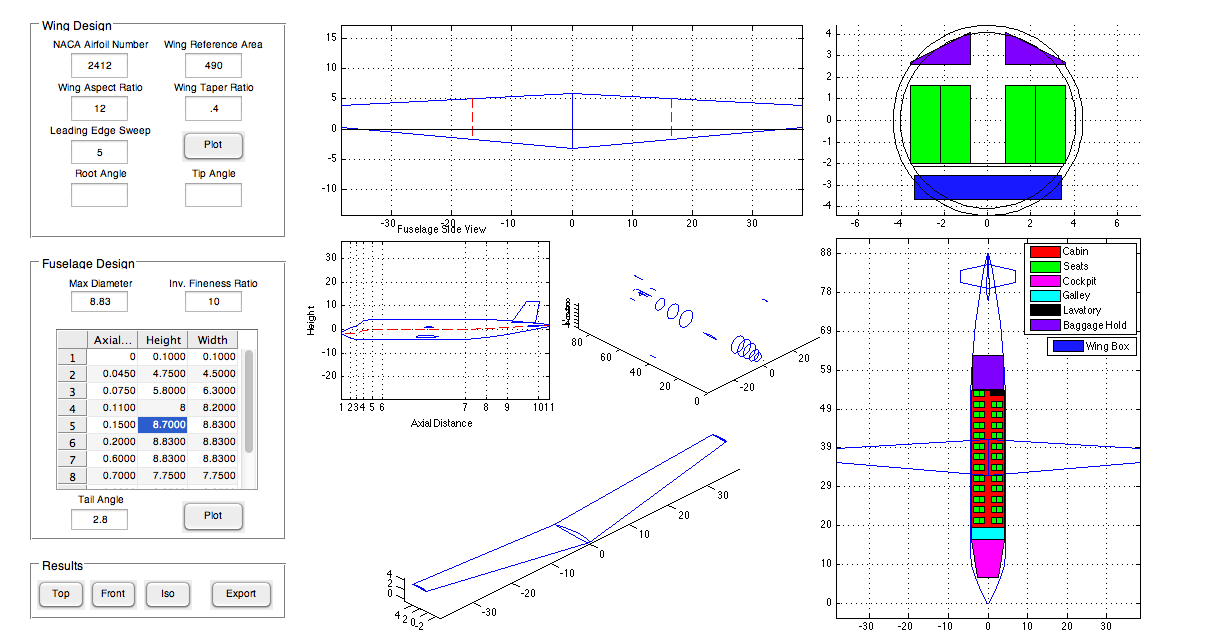
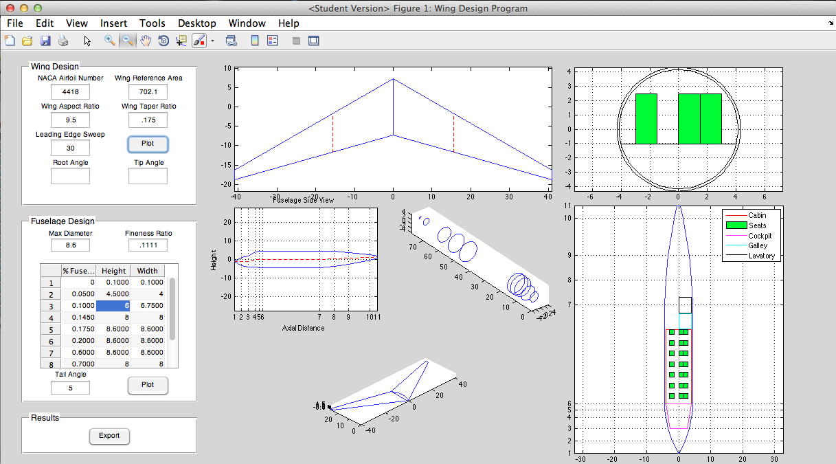
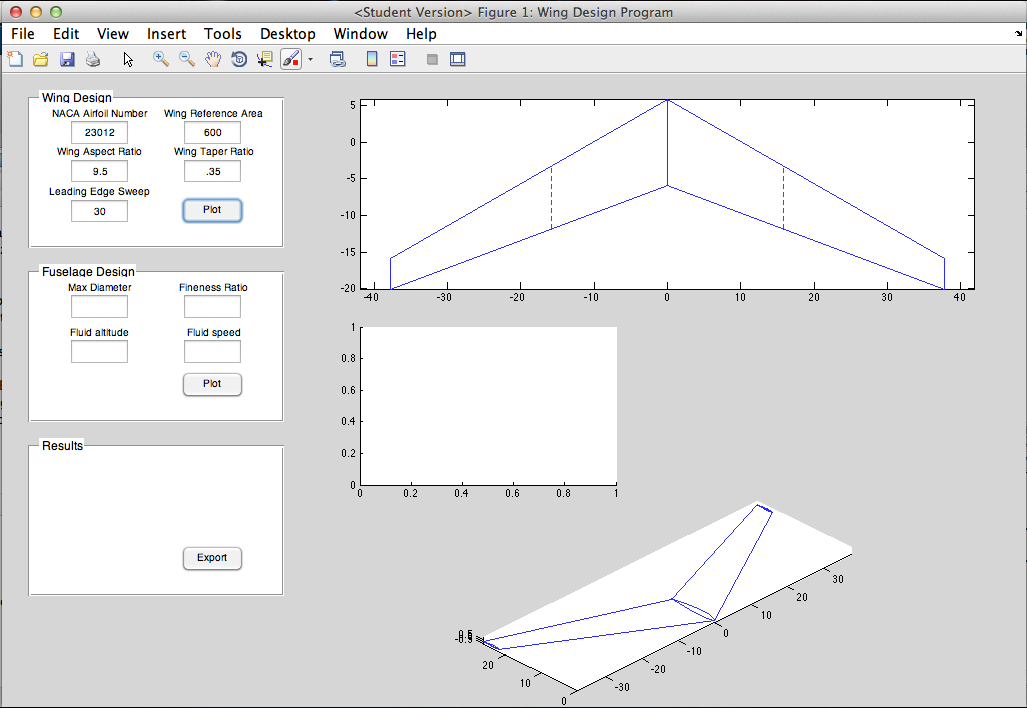
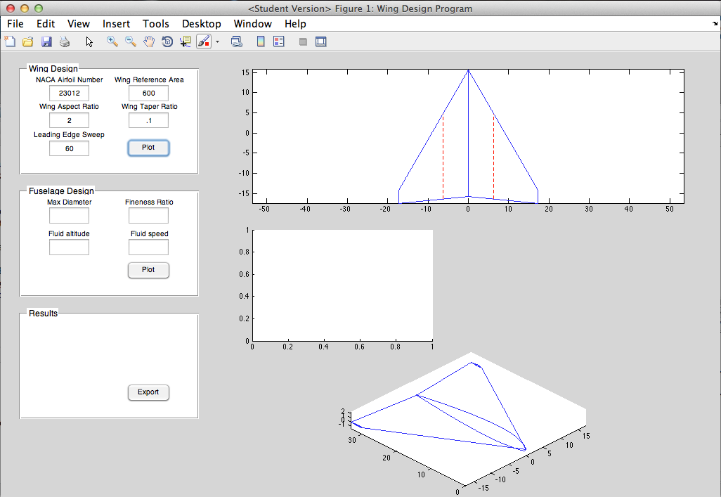
This semester I am taking an aircraft design and performance class. The term project is to complete a conceptual aircraft design - each group will be designing a different type of aircraft. Our group is designing an MSA, or Maritime Surveillance Aircraft. The purpose of this aircraft is to loiter for long periods of time at low altitudes to observe/monitor maritime vessels, act as an airborne control center for nearby aircraft, and even deliver payloads (sonobuoys) and ordnance (torpedoes, air-surface missiles). Our professor provided us with Excel spreadsheets that have many of the calculations programmed into them; our goal is to optimize the parameters to meet the requirements. We also need to produce a 3-D model of our design. This is where the Excel sheets lack in ability. They provide very rudimentary 3-views of the aircraft. I decided to use MATLAB to take the results from the Excel spreadsheet and produce coordinates for a wireframe model of the airplane, which could be loaded into CAD software and turned into a 3-D model.

Currently, my MATLAB program can only produce the wireframe of a wing (or any similar aerodynamic surface). I am actively working on expanding it to create fuselage cross sections which will be used to create a 3-D model.


Design

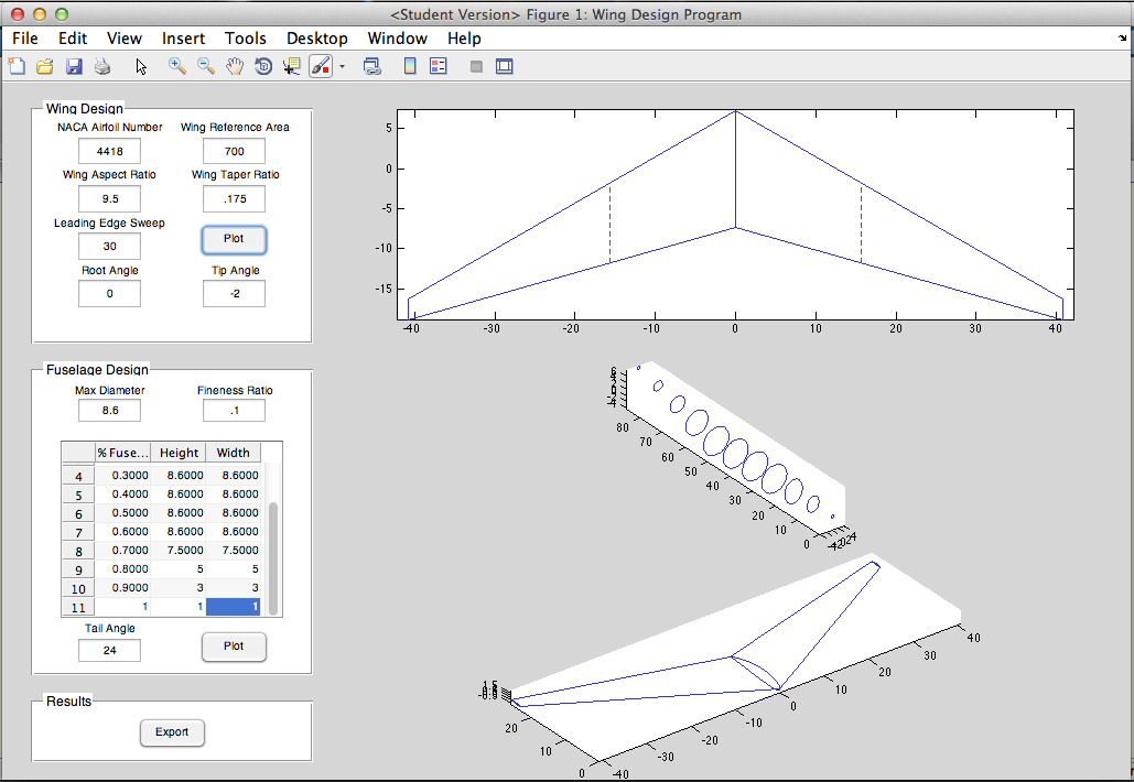
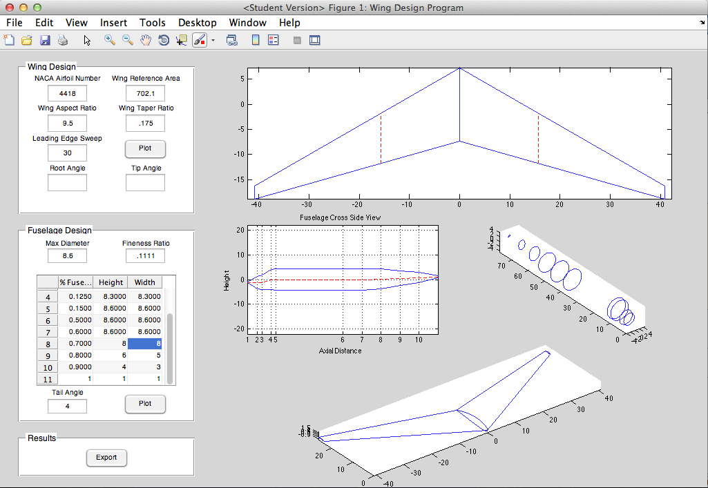
I adapted this program for one I previously made for an aerodynamics class. The inputs were reversed - for that class, the area needed to be calculated for a given wingspan, whereas in the design scenario the wingspan is determined by the area and the aspect ratio, so the inputs needed to be changed. I also added the capability to sweep the wing. I also added the a section on the planform view to show the MAC - this is an important thing to visualize. The 'Export' button creates .txt files with the tip and root airfoil coordinates. These can be loaded into SolidWorks or any other CAD program as a curve, and the tip and root curves can be lofted together into a solid wing. Then the wing is simply mirrored about the root to create the other half and complete the wing.


Capabilities

Plot any 4-digit or 5-digit airfoil (uses my airfoil generator function). Create basic trapezoidal aerodynamic surfaces with airfoil cross sections. Wing twist or washout, and angle of incidence (not visible in GUI yet). Parameters include NACA airfoil, wing reference area, aspect ratio, taper ratio, and LE sweep. Plots MAC and spanwise location of MAC. Export coordinates of root and tip airfoils to create a 3-D model in CAD software.


Improvements

The current method in which the wing is swept is inaccurate, as it 'drags' the tip rearwards (or forwards) to achieve the required leading edge sweep. However the wing should really be rotated such that the airfoils are no longer parallel to the airstream; this is what makes a swept wing effective. Rotating is difficult though, because then you have to account for the fact that tip and the root will be at the incorrect angle, and you have to adjust for that. This is okay to make a model for viewing/aesthetics, but I should look into updating this in the future.  I should also plot points on the quarter chord MAC as this is another important location. I will continue working on this GUI to add fuselage plotting capability. Also the wing washout/twist/angle of incidence parameters can only be accessed from within the code; I need to make boxes on the interface to change these parameters.
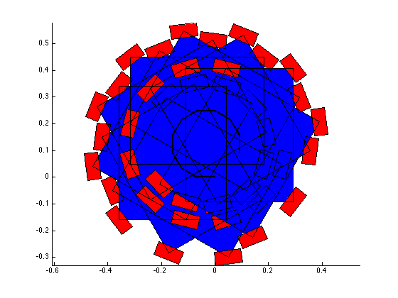
$\setCounter{0}$
In Academic Projects, MATLAB Projects Tags Aircraft Design, MATLAB, Airfoil, Wing Design
1 Comment
  This is an analysis of some actual data from the accelerometer. The filter's effectiveness can be seen in the magnitude spectrum plot in the reduction of both noise and offset. 

This is an analysis of some actual data from the accelerometer. The filter's effectiveness can be seen in the magnitude spectrum plot in the reduction of both noise and offset. 

 This is the same data, but with #nofilter. I'm currently designing a hardware filter to replace the MATLAB filter so I thought a toggle button would be useful. As you can see, without filtering out the noise and the offset, the data make n

This is the same data, but with #nofilter. I'm currently designing a hardware filter to replace the MATLAB filter so I thought a toggle button would be useful. As you can see, without filtering out the noise and the offset, the data make no sense. 

MATLAB Project: Accelerometer Position Transducer GUI

April 13, 2015

For my Instrumentation class, we were tasked with determining the position of a mass on a mechanical oscillator using a transducer. We chose the accelerometer, which is the most difficult transducer to use compared to the others because it has a 2nd order response. Thus, a lot of signal conditioning steps need to be applied to the output of the transducer to find the actual displacement.

Originally, each signal conditioning step was its own MATLAB script. But because the scripts all had different authors, it was difficult for any one of us to go from start to finish with a set of raw data. My solution to this problem was to create a user interface that would allow us to quickly and easily analyze sets of data. The data acquisition would remain its own script and the raw data was saved as a MATLAB data file. The filename is then entered into the GUI and the data is loaded. The static sensitivity of the accelerometer (obtained via calibration) can be entered into the box, but the value from our calibration is already set as the default. The 'Analyze' button does several calculations and makes a few different plots.

The first plot made is just the raw data. The second plot is the magnitude spectrum of the data, so the frequency of our signal and of any noise can be identified. Then the data goes through a bandpass filter to remove the high frequency noise and the DC offset. This filtered voltage as well as its FFT are then plotted. Finally, the signal goes through a double numerical integration to convert the acceleration values into displacement. Because of the cumulative integration technique used, a high pass filter is needed in between integration steps to remove the offset.

Overall I'm quite pleased with how it turned out. I may add more functionality to achieve more of the project's deliverables, but for now this will do.

EDIT: Final Project Report

$\setCounter{0}$
In Academic Projects, MATLAB Projects Tags MATLAB, Instrumentation
Comment

Blogpost Search

Blogposts by Category

Select Category
  • Academic Projects
  • Aviation
  • BreakerBot
  • Engineering Education
  • Illusionist's Locket
  • MATLAB Projects
  • Machining Projects
  • Personal Projects

Archive

  • May 2024
  • December 2019
  • November 2019
  • September 2019
  • April 2017
  • January 2017
  • August 2016
  • May 2016
  • April 2016
  • March 2016
  • February 2016
  • January 2016
  • November 2015
  • October 2015
  • June 2015
  • April 2015
  • February 2015
  • January 2015

Copyright © David Miller 2019