
Background and Theory of Go/NoGo Gages
The use of Go/NoGo gages is quite prevalent in any type of manufacturing environment. Essentially Go/NoGo gages are representations of the respective maximum and least material conditions (MMC/LMC) of a feature. These physical representations of the MMC/LMC are then mated with the feature to assess its quality.
For example, if you think about a simple plug gage, the Go side must fit into the hole to pass. If the hole is too small (exceeds MMC) the Go gage will not fit and the part will fail. Conversely, the NoGo gage must not fit in the hole to pass. If the hole is too large (exceeds LMC) the NoGo gage will fit and the part will fail.
In theory, this principle seems quite straightforward. However the rose colored glasses are shattered when it is revealed that the gages, just as the features they intend to assess, are imperfect. Thus the gages themselves must then have tolerances. This tolerance, known as a gagemaker’s tolerance, is typically around 10% of the feature tolerance. The 10% is then split evenly among the Go/NoGo gages. For example, on a 2.000+/-.005 dimension, the gagemaker tolerance would be .001, and the tolerance for each the Go and NoGo gage would be .0005.
The only remaining question is the bias of the tolerance. The typical bias selected is the most conservative; i.e. it is more conservative to risk rejecting good product than to risk accepting bad product. This will result in the Go gage tolerance range being just within the feature tolerance range, and the NoGo gage tolerance range being just outside the feature tolerance range.
So just as your product has a yield, the gages themselves will also have a yield expressed as False Rejections/Total Rejections. Obviously if the gage is your only way to assess the feature, you will never identify any False Rejections, so a 3rd party measurement some orders of magnitude more accurate than the gage would be needed to make this determination.
Problem Statement
Gages are typically designed/selected based on this 10% rule. I haven’t really found any background on where this originated, or if there is any statistical theory justifying it. From what I have found, it is more of an empirical finding that the 10% rule maximizes yield while keeping gage costs manageable.
What I am interested in is the statistical theory behind this gaging process. In other words, is it possible to analytically calculate the probability of these False Rejections? If this were possible, one could better justify their gage design/selection, or possibly improve yield or reduce gage costs for a given application with knowledge about the distribution(s).
Assumptions
For this analysis, I have made the following assumptions.
All random variables are normally distributed.
The means of the gages’ random variables are at the center of their respective tolerance ranges.
I’m using this assumption in lieu of having any actual information on the distributions of gages.
All gages are made with 6Sigma manufacturing processes.
I’m using this assumption in lieu of having any actual information on the distributions of gages.
Analysis
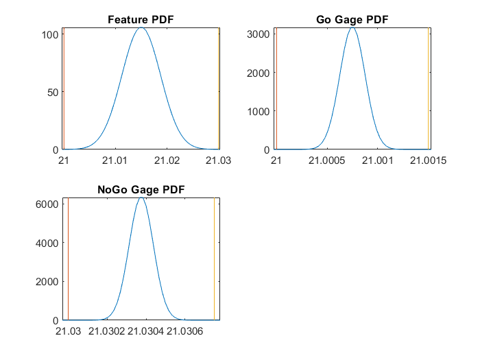
Let A be a random variable describing the dimension of the feature. Let G be a random variable describing the dimension of the Go gage. Let N be a random variable describing the dimension of the NoGo gage.
For an internal feature, the Go gage passes when it fits inside the feature, i.e. A>G. The NoGo gage passes when it does not fit inside the feature, i.e. A<N. Thus we obtain the following:
P(Pass_Go) = P(A>G)
P(Pass_NoGo) = P(A<N)
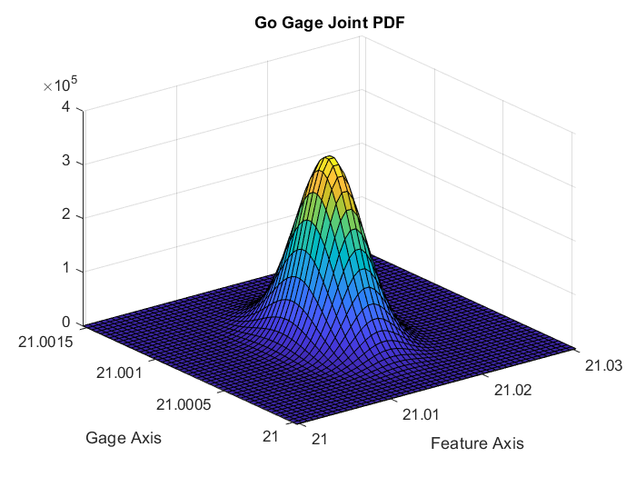
The probability P(A>G) may be obtained by double integrating the joint PDF, F_AG(a,g). Because the feature dimension and the gage dimension are independent, the joint PDF may be expressed as the product of the individual PDFs.
F_AG(a,g) = F_A(a) * F_G(g)
Next we must double integrate this expression. Before integrating, we must understand the space we are integrating in. This joint PDF occupies (a,g) space. Each point on the (a,g) plane represents a combination of the dimension of the feature (a) and the dimension of the gage (g). We are only interested in the case where a>g, and both a>0 and g>0. If a is taken to be the horizontal axis and g the vertical axis, this corresponds to the area under the curve a = g (Fig. 1).

Figure 1
Matlab Script
I wrote a simple Matlab script to visualize the joint PDF. The next step is determining how to evaluate the double integral over this shaded region. I don’t think there will be an analytical solution, so barring that option the next logical alternative is numerical integration. However I’m not sure how numerical integration works over semi-infinite regions such as this one.